


Solar storage system loss analysis: 2026 guide
Discover the essentials of solar storage system loss analysis. Learn how to enhance efficiency and maximize your solar investment in our 2026 guide.
Solar storage system loss analysis is the systematic evaluation of all energy losses occurring during charging, storage, and discharge in a solar battery system. It is the foundation of any credible performance or financial assessment. Modern LFP systems achieve DC round-trip efficiency of 95%–98%, yet full-system AC round-trip efficiency typically falls to 85%–94% once conversion, standby, and thermal losses are included. That gap is not a rounding error. It is the difference between a project that meets its financial model and one that quietly underperforms for two decades. For engineers and energy analysts working across residential and vehicle applications, closing that gap starts with understanding where the losses actually occur.
What are the main types of losses in solar storage systems?
Loss analysis begins at the cell level and works outward through every conversion stage to the point of interconnection. Each layer adds inefficiency, and the cumulative effect is what separates datasheet performance from real-world output.
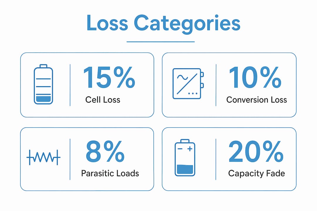
Cell-level losses arise from internal resistance within the battery cells. During charge and discharge, resistance converts electrical energy to heat. Lithium iron phosphate chemistry minimises this compared to older chemistries, but battery cell behaviour still contributes measurable losses, particularly at high C-rates.
Power conversion system (PCS) losses occur at every DC-to-AC and AC-to-DC conversion. Each conversion stage carries an efficiency penalty. In AC-coupled architectures, solar generation passes through an inverter, then the battery charger converts it again to DC for storage, then back to AC on discharge. Three conversions where a DC-coupled system needs one.
Parasitic and auxiliary loads are the most underestimated loss category. Battery management systems, cooling fans, communication modules, and standby inverter draw all consume power continuously. Parasitic loads can account for 8–13 percentage points below conversion efficiency. In low-utilisation scenarios, auxiliary consumption can dominate total system losses entirely.
Thermal losses result from heat generated during charge and discharge cycles. Active cooling systems remove that heat but consume additional power in doing so. Poorly managed thermal conditions also accelerate degradation, compounding losses over time.
Degradation and capacity fade represent the long-term loss dimension. Stationary LFP storage shows approximately 20% capacity fade over 10–12 years, with around 4.5% loss over 490 cycles. That progressive reduction in usable capacity directly reduces the energy available for self-consumption or export year on year.
Pro Tip: Map each loss category separately before aggregating. Analysts who jump straight to a single round-trip efficiency figure miss the parasitic load contribution entirely, which is the most controllable loss in a well-designed system.
How to measure and quantify energy losses at system level
Accurate solar energy loss evaluation requires a structured measurement framework. The industry uses several distinct metrics, and conflating them produces errors in both technical assessments and financial models.
-
Distinguish DC from AC round-trip efficiency. DC round-trip efficiency measures energy in versus energy out at the battery terminals. AC round-trip efficiency measures at the grid connection point and includes all conversion and auxiliary losses. Always specify which figure is being used and why.
-
Calculate the System Performance Index (SPI). The SPI aggregates conversion, control, and standby losses into a single normalised metric. Top residential storage systems reach up to 97.0% SPI. Lower-performing systems show a wide spread, driven primarily by standby consumption and control strategy, not battery chemistry.
-
Monitor auxiliary loads separately. Install sub-metering on BMS, cooling, and communications circuits. This isolates parasitic consumption from conversion losses and identifies which auxiliary systems are the primary efficiency drain.
-
Apply cycle profiling for degradation tracking. Log charge and discharge depth, C-rate, and temperature for every cycle. Plotting capacity against cumulative cycle count produces a degradation curve that feeds directly into long-term financial projections.
-
Use calibrated instrumentation. High-accuracy power analysers with logging capability are the standard tool for field measurement. Data acquisition systems that record at one-second intervals capture the low-power inverter inefficiency that averaged data masks.
The table below summarises the key metrics used in a complete renewable energy performance analysis:
| Metric | What it measures | Why it matters |
|---|---|---|
| DC round-trip efficiency | Battery terminal energy in vs out | Baseline cell and BMS performance |
| AC round-trip efficiency | Grid-point energy in vs out | True system efficiency for financial modelling |
| System Performance Index (SPI) | Aggregated system losses normalised | Benchmarking across different architectures |
| Capacity fade rate | Usable capacity loss per cycle or year | Long-term revenue and savings projection |
| Standby power draw | Auxiliary consumption at idle | Identifies parasitic loss contribution |
What strategies reduce losses and improve system performance?
Energy storage system optimisation operates at three levels: architecture selection, component specification, and operational control. Each level offers distinct efficiency gains.
Architecture: DC-coupled vs AC-coupled. AC-coupled systems suffer from multiple DC-to-AC conversions, causing higher energy losses compared to DC-coupled designs. For new installations where loss minimisation is a primary criterion, DC-coupled architecture is the technically superior choice. Retrofitting existing AC systems is a different calculation, but the conversion penalty must be explicitly modelled.
Component selection criteria:
- Select PCS units with published efficiency curves across the full operating range, not just peak efficiency figures.
- Prioritise LFP chemistry for its combination of low internal resistance, thermal stability, and cycle life.
- Specify BMS units with low standby draw. The difference between a poorly specified and a well-specified BMS can be several watts of continuous consumption.
- Choose power electronics rated for the actual operating range of the system, not the theoretical peak. Oversized inverters run at low load fractions and lose efficiency disproportionately.
Thermal management. Passive thermal management reduces cooling energy demand compared to active fan-based systems. Where active cooling is required, variable-speed fans controlled by temperature sensors consume significantly less power than fixed-speed alternatives.
Intelligent control and forecasting. Predictive dispatch algorithms that use weather forecasting and load profiling keep the system operating in its high-efficiency band. Avoiding very low state-of-charge and very high charge rates reduces both conversion losses and degradation rate simultaneously.
Pro Tip: Run the system’s inverter efficiency curve against your actual load profile before specifying. A unit with 97% peak efficiency that drops to 88% at 10% load is a poor fit for a self-consumption-heavy residential profile.
How do loss factors impact financial viability?
Efficiency is not a technical specification that sits separately from financial modelling. Efficiency differences widen financial outcomes over the asset life, making round-trip efficiency a key economic variable, not just a performance metric.
The compounding mechanism works as follows. A system with 90% AC round-trip efficiency delivers 10% less usable energy per cycle than a 98% DC-only figure suggests. Over thousands of cycles across a 20-year asset life, that difference accumulates into a substantial reduction in self-consumption value and grid export revenue. As electricity tariffs rise over time, each percentage point of lost efficiency costs progressively more in absolute terms.
Capacity fade compounds the problem further. Lithium battery lifespan factors including temperature, depth of discharge, and cycle rate all accelerate degradation. A system that loses 20% capacity over 12 years delivers proportionally less value in its second decade, precisely when the capital cost has been largely recovered and returns should be strongest.
Overlooking standby and parasitic power consumption leads directly to overstated savings in financial models. Auxiliary system power can reach roughly 5–10 kW for a 4 MWh battery. That continuous draw reduces net energy delivered and must appear as a cost line in any credible NPV calculation.
Accurate loss modelling is not a refinement for large commercial projects. For residential systems where margins are tight and payback periods span a decade, a 3% efficiency error in the financial model can shift a project from viable to marginal.
The practical implication for bid evaluation: require AC round-trip efficiency figures, SPI data, and published degradation curves from every system under consideration. Reject datasheets that present only DC efficiency at peak operating conditions.
What are the common pitfalls in loss analysis and system evaluation?
Even experienced analysts make systematic errors in solar system efficiency assessment. The most damaging pitfalls share a common cause: using simplified metrics where the situation demands granular data.
-
Relying on DC-side datasheets alone. DC round-trip efficiency figures exclude AC conversion losses and all parasitic loads. Datasheet DC figures are often misleading without including AC-side and parasitic losses. A system quoted at 97% DC efficiency may deliver 88% at the AC meter.
-
Accepting peak efficiency as representative. Inverters and PCS units publish peak efficiency at a specific load fraction, typically 50%–75% of rated capacity. Efficiency varies by operating mode, and low-power operation common in residential self-consumption profiles can reduce actual efficiency substantially below the published peak.
-
Ignoring standby consumption in low-utilisation periods. A system that sits idle for extended periods still draws auxiliary power. In seasonal or part-time applications such as campervans and motorhomes, standby losses can represent a disproportionate share of total annual energy loss.
-
Applying a single efficiency figure across all operating modes. Loss analysis must reflect the actual usage profile. A vehicle application with frequent partial cycles and variable ambient temperature has a fundamentally different loss profile from a residential system with predictable daily cycling.
Pro Tip: Combine laboratory measurements with annualised system simulations using the SPI framework. Lab data gives you component-level accuracy; simulation gives you the usage-weighted annual efficiency figure that actually appears in the financial model.
Key takeaways
Accurate solar storage system loss analysis requires AC round-trip efficiency data, SPI benchmarking, and explicit parasitic load accounting to produce reliable performance and financial projections.
| Point | Details |
|---|---|
| AC efficiency is the correct metric | DC round-trip figures exclude conversion and auxiliary losses; always use AC figures for financial modelling. |
| Parasitic loads are significant | BMS, cooling, and standby draw can account for 8–13 percentage points below conversion efficiency. |
| Degradation compounds financial impact | LFP capacity fade of approximately 20% over 10–12 years reduces long-term savings progressively. |
| Architecture choice affects losses | DC-coupled systems avoid multiple conversion steps and deliver higher real-world efficiency than AC-coupled designs. |
| SPI enables reliable benchmarking | The System Performance Index aggregates all losses; top residential systems reach 97.0% SPI. |
Where loss analysis is heading: a practitioner’s view
The most significant shift I have observed in recent years is the move away from datasheet trust towards real-world measurement. Engineers who built financial models on DC efficiency figures from 2018 are now reconciling those projections against metered data, and the gaps are instructive. The industry is slowly accepting that performance gaps between systems stem from conversion strategy and standby energy use, not just battery chemistry. That is a more useful frame for system selection.
Silicon-carbide power electronics are the most technically significant development on the horizon. SiC-based inverters and PCS units offer meaningfully higher conversion efficiency across a wider load range than conventional silicon-based designs. For self-consumption-heavy residential profiles where low-load operation is common, the efficiency improvement at partial load is particularly relevant.
The standardisation gap remains the most frustrating obstacle. Without a mandatory reporting framework that requires AC round-trip efficiency and SPI figures alongside DC specifications, procurement decisions will continue to be distorted by selectively presented data. The HTW Berlin Energy Storage Inspection methodology is the closest the industry has to a credible independent benchmark, and its annual findings consistently reveal a wider efficiency spread than manufacturers’ literature suggests.
My practical recommendation: treat loss analysis as a continuous process, not a pre-commissioning exercise. Metered data from the first 12 months of operation should feed back into the financial model and inform maintenance scheduling. Systems that are monitored closely perform better over their full asset life.
— John
Skyenergi’s solar storage solutions for efficient, low-loss systems
Engineers and analysts who have completed a thorough loss analysis need components that perform to specification across the full operating range.

Skyenergi supplies the Victron Energy Solar Home System 200 MPPT, a fully integrated solution combining MPPT charge control with storage management in a single architecture. The integrated design reduces conversion steps and auxiliary complexity, directly addressing the loss categories covered in this guide. For analysts specifying residential or off-grid systems, Skyenergi’s range of Victron MPPT solar panel kits provides a well-matched generation and storage pairing with published efficiency data across the operating range.
FAQ
What is AC round-trip efficiency in a solar storage system?
AC round-trip efficiency measures energy delivered at the grid connection point relative to energy drawn from the grid to charge the battery. It includes all conversion, standby, and auxiliary losses, making it the correct metric for financial modelling.
How do parasitic loads affect battery storage efficiency?
Parasitic loads from BMS, cooling fans, and standby electronics can reduce effective system efficiency by 8–13 percentage points below the conversion efficiency figure. In low-utilisation applications, they can represent the dominant source of energy loss.
What is the System Performance Index and how is it used?
The System Performance Index aggregates conversion, control, and standby losses into a single normalised figure. Top residential systems reach 97.0% SPI, and the metric enables direct comparison across different system architectures and chemistries.
How does LFP capacity degradation affect long-term financial projections?
Stationary LFP storage shows approximately 20% capacity fade over 10–12 years. That progressive reduction in usable capacity reduces annual self-consumption value and must be modelled explicitly in any NPV or ROI calculation covering the full asset life.
Why does system architecture affect energy storage system optimisation?
DC-coupled systems avoid repeated DC-to-AC and AC-to-DC conversions, reducing total conversion losses compared to AC-coupled designs. For new installations where efficiency is a primary criterion, DC-coupled architecture delivers measurably better real-world performance.
Recommended
Prev post

Commissioning lithium battery systems checklist: 2026 guide
Updated on 28 June 2026
Next post

Explain parallel battery banks: a DIY guide
Updated on 26 June 2026


